Anúncios
You’ll find clear, practical insight on how natural areas bounce back after a disturbance. This short introduction explains what scientists mean by a post-disturbance stable state and how a mono-exponential model turns scattered field data into useful timelines you can use in the United States.
You’ll see why carbon fluxes often return within a few decades (~23 ± 5 years in one synthesis of 77 chronosequence case studies), while structural pools like aboveground biomass may need a century or more to approach the stable state.
The same work shows drought can shorten the path back for some functions, while storms may lower the post-disturbance stable level by about 28.2% in forests.
What this gives you is a way to benchmark progress with measurable milestones, set realistic timelines, and choose actions that deliver the best ecological and budget outcomes over time.
Why ecosystem recovery speed matters right now
When droughts and fires occur more often, knowing how long sites take to bounce back becomes essential. Disturbance frequency is rising across the United States, and that shift alters terrestrial carbon balance and service delivery.
Anúncios
Quick rebounds help forests regain sink strength and widen seasonal CO2 swings that scientists track. Major droughts in North America and Europe have already flipped regions from sink to source for years.
“Global fire emissions still add roughly 4 Pg C each year, so the window for net carbon uptake matters for budgets and planning.”
Use recovery time to prioritize action: you can triage sites where function returns fast, sequence tougher restorations later, and design monitoring that flags stalled trajectories early.
Anúncios
- Shorten the carbon-source interval by targeting fast-return areas first.
- Link measurable, time-bound outcomes to funding and reporting.
- Reduce vulnerability to invasives and erosion by acting where rebounds are likeliest.
Bottom line: understanding return timelines helps you manage impacts from frequent disturbance and align work with realistic, fundable goals.
What you mean by ecosystem recovery speed
Think of recovery time as a measurable pace that tells you how quickly a damaged site regains key functions or settles into a new, steady state. This definition is field-ready and easy to apply in monitoring plans.
A practical definition you can use in the field
Use a simple rule: the rate at which a community and its environment return to a pre-disturbance state or settle into a new, stable state. Anchor that rate to measurable variables such as carbon fluxes, LAI, and aboveground biomass.
How it signals ecological resilience and sustainability
Faster return indicates stronger capacity to absorb shocks and restore function. Slower or partial return flags greater ecological consequences and longer service gaps.
Translate the metric into operations: set monitoring intervals, define intervention thresholds, and compare treatments across sites. Use the same variables and time windows so your information stays consistent and stakeholders share realistic expectations.
- Measure: pick 3–5 variables and a time unit (years).
- Compare: rank sites by rate and choose actions that accelerate trajectories.
- Report: state clear targets for what counts as meaningful recovery on practical time scales.
Signals from recent studies: recovery is faster in some systems than you’d expect
Recent syntheses point to a clear pattern: functional measures often rebound sooner than structural pools after a major disturbance. That split shapes what you can expect when planning monitoring and restoration in the United States.
Evidence from the terrestrial carbon cycle
A broad study of 77 chronosequence cases fitted a mono-exponential rise to a post-disturbance stable state (95% threshold).
Forest carbon fluxes returned in about 23 ± 5 years, while aboveground and total biomass commonly needed 100+ years to approach that same state.
When “full recovery” is realistic — and when a new state appears
Many variables reached post-disturbance levels similar to pre-disturbance values. In forests, LAI and NPP often overshot by ~10% and ~35%, signaling vigorous regrowth.
Droughts tended to show the shortest rebounds, whereas storms lowered post-disturbance stable levels by ~28.2% in some forests. That means you may see functional return fast, yet structural change can lag for decades.
- Practical: use the 95% endpoint to set monitoring targets.
- Plan: expect quick functional wins but allow long timelines for biomass rebuild.
- Read more: consult a synthesis study for methods and case details.
Inside the asymmetric response concept: five recovery trajectories shaping outcomes
The Asymmetric Response Concept (ARC) lays out five clear trajectories that communities can follow after a major disturbance.
This framework helps you predict which path a site will take and plan actions that match the likely outcome.
Rubber band vs. broken leg: complete recovery on different timescales
Rubber band sites bounce back fast and regain their prior state in short time frames.
Broken leg sites also reach the same state, but it takes decades or longer because key species return slowly.
Partial, no recovery, and new state: when communities don’t bounce back
Partial outcomes occur when some functions or species fail to return without help.
No-recovery cases show stalled trajectories and clear ecological consequences.
New state means different species fill roles and you must redefine success for that site.
Why tolerance, dispersal, and biotic interactions decide the path
Who survives the stress matters: species tolerance sets the starting point for reassembly.
Dispersal governs whether species can return naturally; you may need assisted movement or nearby sources.
Biotic links—predators, mutualists, hosts—often control whether reintroductions succeed.
- Compare rubber band and broken leg to set realistic time and budget plans.
- Watch for warning signs of partial or no recovery and act early.
- Sequence reintroductions to match food-web needs and avoid wasted effort.
How models quantify recovery time and state change
Simple mathematical fits let you trace a variable’s rise from disturbance to near‑stability with practical precision. That clarity matters when you must set targets, budgets, or monitoring plans across the United States.
The mono-exponential rise to a stable state
The mono-exponential model fits a rise‑to‑maximum curve to scattered field points. It yields an intercept, a rate, and an asymptote that represents the post‑disturbance state.
In one synthesis, researchers fitted 191 models across 77 case studies. About 25 fits had low R² (
From pre-disturbance to post-disturbance stable state: defining “95% recovered”
Define recovery time when a variable reaches 95% of the post‑disturbance state. Use undisturbed controls or old‑growth values as pre‑disturbance baselines to measure change over the period.
- Compare consistent variables to identify reliable leading indicators.
- Plan monitoring frequency and spatial scales so the model captures the rise.
- Report uncertainty ranges to justify timelines in grants and compliance documents.
“quotes,”
Ecosystem recovery speed: what the timelines look like by variable
Different variables trace different timelines; you’ll see quick functional returns and much slower biomass gains. Use these ranges to set realistic monitoring and budgets for United States sites.
Fast responders—carbon fluxes, NPP, and LAI—often reach a new stable state in decades.
Fast responders
Carbon fluxes typically approach stability in about 23 ± 5 years. Gross primary and net primary productivity follow: NPP centers near 32 ± 13 years, while LAI sits near 42 ± 17 years. These variables are your best early indicators of functional rebound.
Slow responders
Structural pools take far longer. Aboveground, belowground, and total biomass commonly need ~96–104+ years. Soil and litter carbon require at least ~60 years. Plan multi-decadal to century-scale monitoring if your goal is stock restoration.
Middle lane indicators
Microbial C and species richness fall between function and structure. Microbial carbon averages ~52 ± 18 years, and species richness near ~86 years. Tracking these helps flag stalled trajectories before structural pools show change.
- Actionable: prioritize fluxes and primary productivity to confirm early wins in decades rather than centuries.
- Plan: budget for longer recovery time for biomass and soil pools.
- Design: set variable-specific targets and include confidence ranges when reporting progress.
Disturbance matters: drought, fire, harvest, mining, storms, and deforestation
Different disturbances set very different clocks for return. Your plan should start by ranking the type of disturbance so you can triage sites for near‑term gains and long‑haul work.

Shortest recoveries: drought in forests and grasslands
Drought often yields the fastest turns. In many grasslands and some forests, function returns in only a few years.
This quick rebound lets you bank early wins and reallocate effort to tougher cases.
Longer recovery time: harvest and fire vs. mining in forests
Harvest and severe fire in forests commonly exceed eight decades to approach the post‑disturbance state.
Mining sites may need roughly four decades, so they can be better candidates for pilot restoration than some harvest‑impacted stands.
Deforestation and storms: century-scale trajectories for biomass
On average, deforestation requires about 100 years for biomass to rebuild. Plan policy and carbon accounting around that horizon.
Storms can lower the post‑disturbance stable state by ~28.2% in forests. That means even after long recovery time you may not reach prior baselines.
- Rank disturbances by expected recovery time to set priorities.
- Leverage drought’s rapid return for early monitoring wins.
- Budget century‑scale timelines for deforestation and long fire or harvest cases.
- Pilot restoration on mining sites where timelines are often shorter.
- Adjust targets when storms depress the post‑disturbance state.
Severity, state change, and time: the relationships you can expect
Severity often predicts how far and how long a site departs from its prior state. Data show recovery time and the magnitude of state change rise with disturbance severity (P < 0.01), though coefficients are small because outcomes vary by disturbance type and by variables measured.
Higher severity tends to mean longer recovery time
When a disturbance is intense, you should expect extended timelines. In practice, greater severity correlates with longer recovery time across many sites and case studies.
That pattern holds even when variability is high. Treat severity estimates as practical predictors for monitoring and funding.
How magnitude of state change scales with disturbance
Higher-impact events usually produce larger deviations from baseline. Many variables trend back toward similar equilibrium states, but they often take more time to do so after severe disturbance.
- Plan: use severity to set monitoring intensity and adaptive intervention timing.
- Communicate: explain that longer timelines at severe sites are expected, not failure.
- Compare: employ severity-stratified reporting so you compare like with like.
Bottom line: use severity as a simple, actionable predictor to forecast both time and magnitude of change. That helps you align budgets, procurement, and expectations across your portfolio and decide when a new stable state is the realistic endpoint.
When ecosystems recover faster than anticipated: drivers and examples
You’ll find that proximity to intact sources and quick repair of biotic links often shorten timelines dramatically. When nearby populations can disperse into a site, colonization happens faster and community structure rebuilds more quickly. This matters when you set goals and budgets for restoration in the United States.
High dispersal and nearby source populations accelerate rebounds
Target sites near intact habitat to harness natural movement of seeds, larvae, and mobile adults. Where distances or barriers block return, use assisted movement to bridge gaps.
Rewiring biotic interactions: restoring prey, hosts, or mutualists
Sequence actions so prey or host plants arrive before predators or symbionts. Detect and reintroduce missing mutualists — pollinators, mycorrhizae, or cleaners — that quietly limit progress.
- Design: add habitat features and corridors that reduce travel time and boost colonization success.
- Sequence: rebuild food webs in logical order to avoid wasted effort.
- Genetics: integrate source diversity to prevent bottlenecks that slow long‑term stability.
- Timing: align releases with seasonal windows to improve establishment.
- Monitor: track interaction networks, not just single species, to confirm durable gains.
Examples show that simple proximity and smart sequencing can convert partial or stalled trajectories into fast, functional returns. For practical case studies, see restoration examples at this synthesis.
Measuring recovery in practice: the metrics that matter
Start by choosing a small set of indicators that tell you whether the site is regaining function or just looking green. Pick 3–5 variables that span fast fluxes and slow pools so your monitoring shows both early wins and long-term change.
Gross primary productivity, ecosystem respiration, and net exchange
Track gross primary productivity, ecosystem respiration, and net ecosystem carbon exchange to capture early functional return. Use eddy covariance towers, flux chambers, or well‑calibrated remote sensing to get continuous, comparable time series.
These fluxes usually move back toward the post‑disturbance state in decades, so monthly to annual sampling windows work well for near‑term signals.
Tracking biomass, LAI, soil and litter carbon pools over years
Pair flux data with LAI and biomass plots to avoid overestimating long‑term carbon gains. Add soil and litter carbon pools and microbial biomass C to catch slower parts of the carbon cycle.
- Define metric-specific recovery time and a 95% endpoint for each variable.
- Match sampling intervals to variable dynamics: fluxes often need frequent reads; pools require decadal surveys.
- Benchmark against controls and build dashboards that show near-term function and long-term stocks.
“quotes,”
What you can do to speed recovery in U.S. terrestrial ecosystems
Start by removing ongoing stressors. You must eliminate pressures such as pollution, chronic grazing, or altered hydrology before expecting durable gains.
Once stressors stop, sequence reintroductions to rebuild the food web. Restore prey, host plants, or mutualists first, then return predators or obligate species so each release finds the resources it needs.
Remove stressors, then match reintroductions to food‑web needs
Act in order: clear the threat, then reintroduce species that support higher trophic levels. This reduces failed attempts and speeds community assembly.
Design for dispersal: corridors, proximity, and timing
Map source populations and add corridors or stepping stones to shorten dispersal time. Put releases in seasonal windows when establishment odds are highest.
Model‑informed targets: set realistic years‑to‑recover by variable
Use chronosequence models to set variable‑specific targets: expect fluxes to stabilize in decades and biomass pools to take near a century. Align budgets, contracts, and monitoring to those timelines.
- Plan: eliminate persistent stressors first.
- Map: locate sources and install corridors.
- Sequence: rebuild prey/hosts before predators.
- Set targets: use model years for each variable.
- Adapt: adjust actions when monitoring shows stalls.
Work with local partners across the United States to maintain corridors, reduce mortality of reintroduced species, and scale practices to local conditions. Use interim milestones to show progress while longer‑term pools accumulate.
Implications for policy, land management, and industry in the United States
Prioritize projects by likely timeline to deliver visible wins and reduce portfolio risk. Use modelled recovery time to rank sites where functional variables return in decades versus sites that need century-scale work.
Prioritizing projects with shorter time-to-stable-state for near-term gains
Start with sites where the state of key variables rebounds fastest. Drought-impacted parcels and some mined lands often reach functional endpoints sooner.
That allows you to claim early results, attract funding, and free capacity for tougher, long-term cases that need sustained investment.
Incorporating ARC trajectories into restoration planning and reporting
Integrate ARC trajectories into permits, contracts, and monitoring frameworks. Doing so clarifies expected outcomes and aligns timelines across agencies and industry.
- Balance: pair quick-return projects with long-term builds for structural carbon.
- Model: use chronosequence models to set realistic milestones and reduce project risk.
- Align: tie incentives to early functional gains while funding longer recovery for stocks.
- Coordinate: maintain corridors and cross-jurisdiction actions to improve recolonization and reduce delays.
- Publish: make timeline assumptions and updated monitoring information transparent to stakeholders.
Bottom line: you can use these relationships and models to design policies that favor achievable outcomes, while still supporting the longer work needed in many forest ecosystems and places facing larger changes.
How we know: chronosequence syntheses and model fits behind these trends
Chronosequences let you infer long-term patterns by comparing sites of different ages and fitting the same curve to each set of points.
In one central synthesis, authors compiled 77 case studies, extracted chronosequence data, and fitted 191 model curves. That approach reveals clear recovery dynamics across variables and disturbance types.
What 77 case studies tell you about recovery dynamics
You’ll see which variables return fast and which need decades. The synthesis found many post-disturbance stable states near pre-disturbance values, with notable exceptions like LAI and NPP increases after some events.
Limitations to watch: variable sample sizes and low-R² fits
Not every model fit is strong: 25 of 191 fits had R² < 0.4. That means some estimates are directional, not definitive.
- Practice: use case-based ranges to build conservative and optimistic scenarios.
- Method: extract consistent variables and apply the same equations for apples-to-apples comparison.
- Context: sample sizes and disturbance type affect confidence, so tailor results to your site and scales.
“You can replicate these methods to build monitoring targets and justify timelines.”
Conclusion
Set simple, variable-specific targets so you can claim measurable wins in years and decades. Focus first on fluxes and other fast responders, while funding longer work for biomass and soil pools that need decades to a century to approach a new state.
Expect that some ecosystems recover toward pre-disturbance levels, but others settle into a new stable state. Use severity and ARC principles—tolerance, dispersal, biotic links—to choose sites where interventions pay off fastest, and apply lessons from drought-impacted areas to speed early gains.
Track progress with clear recovery time targets, adapt as monitoring updates your plan, and balance short-term wins with commitments to deeper restoration in U.S. forests and other terrestrial ecosystems.